Crowd pleaser: Ensemble modelling for accuracy and explainability

Originally published by The Actuary, 7 March 2024. © The Institute and Faculty of Actuaries.
Click here to read the original article.

Karol Gawlowski , John Condon, Jack Harrington and Davide Ruffini explore how ensembling techniques can help us to combine the strengths of GLMs and Machine learning algorithms (i.e. XGBoost) for improved performance without fully compromising transparency.

Actuaries no longer need to choose between accuracy and explainability when modelling. Ensembling can enhance both.

At the heart of every predictive modelling exercise is the accuracy-explainability dichotomy, which can pull actuaries in different directions. Traditional models such as generalised linear models (GLMs) have long been favoured for their simplicity and transparency, but the quest for better performance has introduced more complex algorithms, such as gradient boosting machines (GBMs).

Practitioners often feel forced to opt for one or the other, depending on whether interpretability or predictiveness is the primary goal. However, the approach need not be so binary: a wide array of architectures combine the two.

Combining multiple model predictions into one is known as ensembling, with ‘bagging’ and ‘boosting’ being the standard techniques. Our goal is to use these combinations to improve predictive performance while retaining as much explainability as possible.

Bagging

Bagging, short for ‘bootstrap aggregating’, involves randomly sampling with replacement from the data, and training a model on each of these bootstrapped samples. For a regression task, the final prediction is the average of all the model predictions.

This idea is not new – the ‘wisdom of the crowd’ concept was first observed by statisticians such as Sir Francis Galton, who witnessed a ‘guess the weight of an ox’ contest at a fair in 1906 and found that the median estimate was within 0.8% of the true weight. The crowd’s success can be attributed to averaging out random errors, assuming independence among individuals.

However, this approach can be undermined by systematic errors. In ensemble models, to reduce the risk of correlation between errors in the constituent models, bagging can be extended to only use a random subset of features when training each bootstrapped model. This approach is a random forest and typically performs better than bagging alone.

Boosting

Boosting builds an ensemble of decision trees sequentially, with each new tree correcting the errors of the previous ones. The chosen optimisation method during the fitting process is gradient descent – hence ‘gradient boosted’. While bagging and random forests achieve random model diversity, boosting creates targeted model diversity, improving performance. Figure 1 shows the process.

Figure-1 - Uncredited For the boosted method, we modelled using XGBoost instead of the vanilla GBM. GBMs tend to have a longer training time than XGBoost because XGBoost implements parallelisation during training. XGBoost also includes regularisation techniques such as Lasso and Ridge or row/column subsampling and various other hyperparameters that prune overly complex and overfitting trees. Other differences include XGBoost’s automatic handling of missing data and more efficient splitting algorithm.

We set the different architectures a common task: predicting the frequency of third-party motor liability claims. The dataset used is publicly available and is commonly used in literature on actuarial models and model benchmarking, comprising 680,000 records and 11 features relating to a French insurer’s motor policies.

Unsurprisingly, XGBoost performed better than the pure GLM when fitting to the data. The logical follow-up was to see if we could improve its performance using the GLM. It turns out that the different XGBoost-GLM ensembles did not outperform XGBoost alone. However, as we will explain, GBM practitioners may have many more uses for these ensembles, and performance improvements could be achieved on other, more varied datasets.

Boosted GLMs

Can we improve the GLM’s predictiveness without losing explainability? Enter GLM + XGBoost: the boosted GLM.

A boosted GLM combines a standard GLM’s strengths with a GBM’s advanced capabilities. First, a GLM captures the main effects, providing interpretability and ease of use. XGBoost then identifies and models any residual patterns missed by the GLM. These are here defined as the difference between the response and the model’s prediction. The models’ outputs can then be added together to give the final prediction.

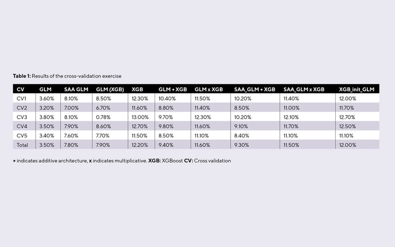
This approach provides improved predictive performance, as Table 1 shows. It also allows actuaries to explain the primary drivers of the model’s predictions to stakeholders, avoiding the black-box nature of purely tree-based models.

Table-1 - Uncredited One point to consider is the risk of overfitting – present with all models, but particularly prevalent when capturing residual patterns. Actuaries must validate the model’s performance on unseen data to ensure its generalisability. Cross validation can be used to ensure a more reliable estimate of model performance compared with using a single train-validation-test split.

In our modelling pipeline, we performed fivefold cross validation. The model was fitted once over three partitions of the data, using one as validation and one as an unseen test. This was done five times, varying the partitions in each iteration.

This ensemble approach used an additive adjustment from XGBoost to improve fit, but a core characteristic of premium breakdowns is their multiplicative nature. Therefore, adding a residual prediction to a GLM may not be the most intuitive approach and may make things harder to interpret.

We can instead use XGBoost to model the ratio of the response variable to the GLM prediction, rather than modelling the residual itself, which may be better at capturing non-linear relationships or complex interactions. Its (GLM x XGBoost) superior model performance can be seen in Table 1 – and it delivers a more coherent and interpretable model. Sometimes you can have your cake and eat it!

Other approaches

We’ve seen how GBMs can help the GLM practitioner, but does it work both ways?

Let us consider a GBM initialised with GLM predictions (XGBoost_init_GLM). The rationale here is that initialising XGBoost with GLM predictions is like starting with a well-drafted sketch (the GLM) that captures a scene’s essence, allowing the artist (GBM) to focus on refining and enhancing the masterpiece.

XGBoost_init_GLM can help the XGBoost algorithm to converge faster towards the best solution because it begins with predictions that are already aligned with the data characteristics. This may not be overly significant for our small dataset, but the savings can be material in bigger modelling exercises. This speed improvement is often accompanied by more predictive accuracy.

It’s like starting with a well-drafted sketch (the GLM) that captures a scene’s essence, allowing the artist (GBM) to focus on refining and enhancing the masterpiece Yet another approach is to use the XGBoost output as a predictor in the GLM. This can improve a GLM’s predictive performance while retaining its transparency. However, the meaning of the GLM coefficients – fitted in the presence of an XGBoost output – is now very different.

For example, in the case of a GLM driver age curve, those relativities would normally represent the influence on the risk attributed to the age factor. However, when XGBoost predictions are included as a covariate in the GLM, the XGBoost predictions will already have used the age information during fitting, so the GLM age relativities are now a closer reflection of how age can reduce the residual after an XGBoost has been fitted. Given that the XGBoost prediction itself is difficult to interpret, the GLM relativities are also less interpretable in this setup.

In our exercise, this ensemble achieved only a very small performance improvement compared with a well-crafted GLM. Not every approach to combine models will result in meaningful improvements, and they can sometimes complicate interpretation without providing significant performance gains.

We also considered how GLM performance affects the ensemble. When examining novel model architectures, authors usually evaluate their proposition against a vanilla GLM. In practice, however, a GLM will have been carefully crafted. For a deep dive on that topic, we recommend the Swiss Association of Actuaries’ (SAA) GLM study, ‘Case Study: French Motor Third-Party Liability Claims’. Its proposed GLM is more performant than a vanilla GLM, but considerably worse than an out-of-the-box XGBoost.

Levelling up: How to close the pensions gap Snapshot: Modern slavery in numbers Modern slavery: Know the regulations Notably, ensembles of XGBoost with a basic GLM outperform ensembles using the superior GLM (SAA_GLM +/x XGBoost). This might be due to the basic model achieving more model diversity with the XGBoost, demonstrating the idea that ensemble models work best when the constituent models are uncorrelated in their residuals – but that is outside the scope of this article.

The final architecture examined was a weighted average of the predictions from both the GLM and XGBoost:

Weighted average prediction = α * GLM prediction + (1- α)*XGBoost prediction where α is between 0 and 1.

The model performed best by solely taking the XGBoost prediction. Neither the basic GLM or the SAA GLM could contribute the model diversity required to generate a predictive improvement when combined with XGBoost. Again, this outcome is specific to our dataset and the models fitted.

watercolour houses - Credit: istock - 1266649316 Results

Table 1 shows the results of the cross-validation exercise. The metric used to assess model performance here is the pinball score, which calculates the percentage improvement in Poisson deviance for each model with a homogenous (mean-only) model as the baseline.

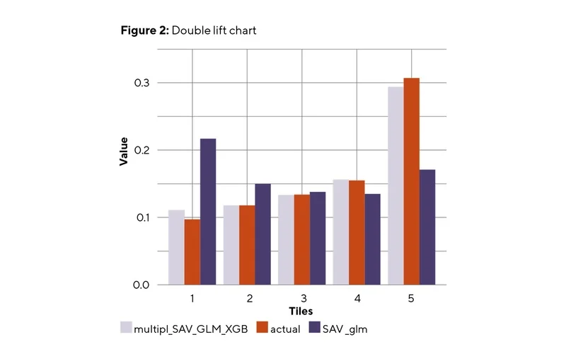
Figure 2 compares the single SAA GLM against the SAA GLM assisted by the multiplicative XGBoost adjustment. The test dataset is divided into quintiles based on the ratio of the two models’ predictions. Each bucket contains both models’ mean actual values and mean predictions. The GBM adjustment’s effectiveness is seen in how closely the ensemble model aligns with the actual values compared to the GLM, indicating more prediction accuracy.

Figure-2 - Uncredited Historical wisdom

If he were around today, Aristotle would likely be a practitioner of ensembling: in his work Politics, he noted that “it is possible that the many, though not individually good men, yet when they come together may be better, not individually but collectively, than those who are so.”

This idea underpins both bagging and boosting, which rely on combining a series of weak learners and result in tree models that are leading the way when it comes to predictive power. It is further demonstrated by the improvement achieved in GLM performance when it is blended with a GBM.

The key to success, however, is model diversity. If diversity is guaranteed, the resulting ensemble can achieve good performance even if the individual models are only slightly better than random guessing, as described in Thomas G Dietterich’s paper ‘Ensemble Methods in Machine Learning’. Sometimes, incorporating less accurate models can enhance the ensemble’s diversity and improve its ability to generalise to new data, as seen in our use of the basic GLM over the developed version.

Practitioners should consider ensembling even though it may increase the modelling workload. It uses the collective strengths of multiple models to achieve better predictive performance, echoing both historical wisdom and modern statistical insights.

Click here to find the full modelling method on GitHub.

Karol Gawlowski is a predictive modeller at Allianz Commercial and chair of the IFoA Actuarial Data Science Working Party John Condon is a lecturer in actuarial science, School of Mathematical Sciences, University College Cork Jack Harrington is an actuarial contractor and predictive modeller at Allianz Personal Davide Ruffini is a pricing actuary at AmTrust Assicurazioni