Supervised learning techniques in claims frequency modelling

Originally published by The Actuary, July 2021. © The Institute and Faculty of Actuaries.
Click here to read the original article.

Neptune Jin shares the Data Science Research Section’s work looking at the merits of different supervised learning techniques for claim frequency modelling.

Using historic data to estimate future claims is a central part of actuarial work, and accurate predictions are essential for risk management. With the development of data science, machine learning techniques have become readily available for improved prediction performance.

Supervised learning models, where algorithms are trained on a labelled dataset to solve classification or regression problems, have wide applications in the insurance industry. Many apply one or more algorithms to boost performance for different purposes – one of which is the prediction of future claim frequencies of policies.

We looked at some of the commonly used supervised learning algorithms – including decision tree, random forest, gradient boosted machine (GBM), neural network and naive Bayes models – and compared their performance when predicting the number of claims for a subset (10% of data, referred to as test or out-of-sample data) of French motor insurance policies (with 90% of data being used for training). We also explored ways to improve performance respectively, showcasing the details and features of each application.

Exploratory data analysis
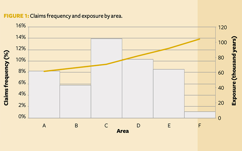
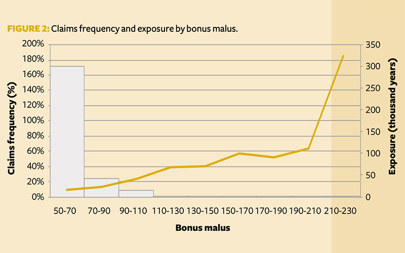
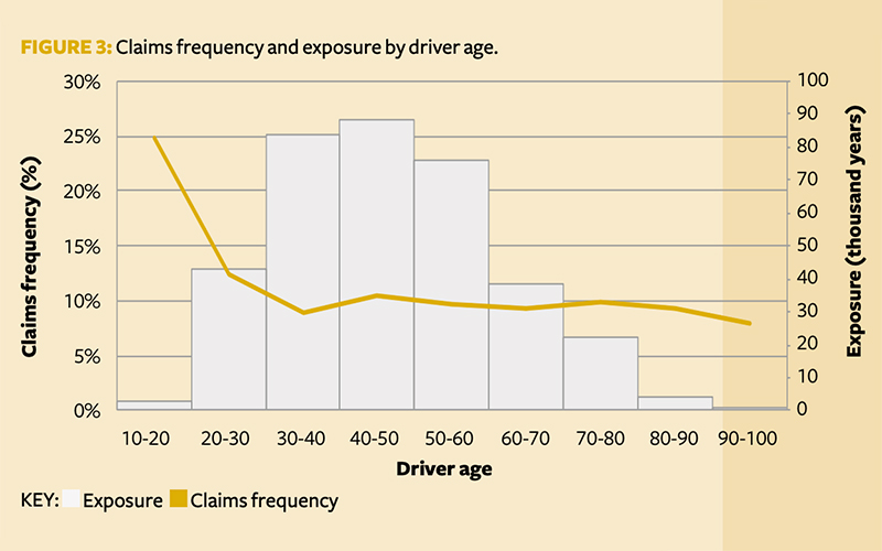
We first explored the claims frequency (observed claims/exposure) and total exposure (length of policy) by feature, with those showing potential predictive capabilities summarised in Figure 1, Figure 2 and Figure 3. The features are:

• Area – Area represents the density value of the city community in which the car driver lives, ranging from ‘A’ (rural areas) to ‘F’ (urban centres). The claims frequency increases as we move from sparse to dense areas (A-F). There is low exposure in Area F, and it could be grouped with E.
• Driver age – There appears to be a decreasing claims frequency trend until the 30-40 age group, where it levels out. This is logical, as younger drivers have less experience. The claims frequency has a slight uptick at the 40-50 age group.
• Bonus-malus – There is very little exposure above 120, but a slight increase in claims frequency is seen with a greater bonus-malus score. Claims frequency could be capped at 120. A logarithmic transformation could be applied to return a normally distributed variable.

The exploratory analysis is used to decide which feature requires engineering. In the case study, this takes the form of binning, capping and logarithmic transformations.

Baseline model
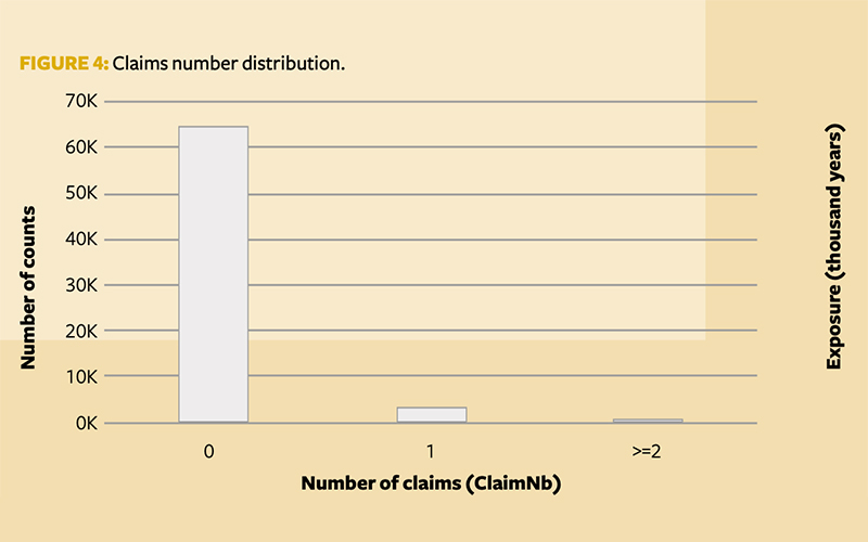
Claims counts observed during the one accounting year of the French motor insurance portfolio show a typical claims count distribution, as shown in Figure 4. This makes the Poisson generalised linear model (GLM) an obvious choice as a baseline model.

However, it is worth noting that ClaimNb (observed number of claims) is highly skewed on zeros and quite sparse beyond value two. To account for this skewness, a traditional Poisson GLM is built alongside a zero-inflated Poisson (ZIP) model.

The ZIP model is a variation of the Poisson GLM commonly used for datasets with excessive zeros. It assumes there are two processes determining the counts: the first determines if a claim occurs or not; if it does, the second determines the number of claims driven by the Poisson probability mass function.

However, the performance of the ZIP model did not show material improvement in this case – at least, not without extra pre-processing of the features, where we used Poisson deviance loss for comparison. The baseline Poisson GLM gave 0.3078, while the ZIP model gave 0.3084 for Poisson deviance loss, which is slightly worse. Although the root-mean-square error (RMSE – the standard deviation of the prediction errors) of the latter is better, we need to keep in mind that it could be the result of populating a lot of zero values.

For simplicity we use RMSE as the metric of performance for the rest of the model illustrations, but the problem of excessive zero values could call for separate research into a proper solution.

Supervised learning models
Categorical variables are one-hot encoded, and numerical ones standardised using a minimum-maximum scalar before each algorithm is fitted. For a fair comparison, all models are fitted to the same transformed dataset.

Tree-based models
Decision trees form the basis of several models in machine learning. At their simplest, a single tree can be used to predict the value of a single variable; this is known as a regression tree, where the predicted outcome can be considered a real number. A random forest model is a form of ensemble learning method where several trees are combined to generate a predicted value. This prediction is an average of the regression trees in the model. The trees in a random forest tend to be weaker learners than a decision tree on its own. However, this weaker learning and averaging effect generally provides a prediction that is more accurate on unseen data than the prediction provided by a single decision tree.

We trained a decision tree and a random forest to predict the ClaimNb in our dataset. The scikit-learn Python library is used here, specifically the tree regressor and random forest regressor models.

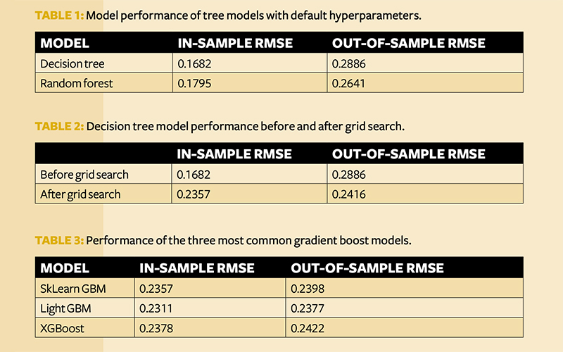
Fitting these models with default hyperparameters, we generated the RMSE seen in Table 1. As expected, the random forest model outperforms the decision tree model on out-of-sample data, demonstrating the strength of ensemble learning when generalising to unseen data.

Next, model parameter (hyperparameter) tuning was carried out using a randomised grid search, with cross-validation for the decision tree model. The model hyperparameters with the best error were then chosen for the candidate model. The performance of the decision tree model illustrates the correcting effect of good hyper-tuning for overfitting.

The grid search is a very time-consuming exercise to run. Table 2 only shows the results of the decision tree search, as a random forest grid search would take even longer.

Before grid searching, a fair bit of overfitting was shown on the model; this was no longer present after the tuning. This shows the importance of identifying the proper parameters in getting models that generalise well.

Gradient boosting machines
GBMs cover a wide variety of algorithms, but only a handful of off-the-shelf models are commonly used. These have become well known within data science fields as they tend to outperform traditional GLM approaches, although they can be susceptible to overfitting.

Gradient boosting derives a strong learner out of a series of weak learners through iteration. It starts with an imperfect model that gives relatively weak predictions (typically a decision tree) and takes the errors/pseudo-residuals back to ‘teach’ the model to be stronger. The updated model gets stronger through an iterative process until it is optimised to produce highly accurate results.

In this study, we trained the following popular gradient boosted decision tree models on the target variable (ClaimNb):

• XGBoost
• LightGBM
• SKLearnGBM

Initially, these models were trained to the dataset with default hyperparameters. It became clear that SKLearnGBM did not generate competitive results, so this model was dropped.

To tune the hyperparameters, an initial randomised grid search was run across a subset of parameters, using a fivefold cross-validation in order to prevent overfitting. The following parameters were varied under the associated models:

• XGBoost – Max depth, learning rate, Alpha (L1 regularisation), minimum child weight, and subsamples
• Light GBM – Max depth, learning rate, Lambda (L1 regularisation), number of estimators, minimum child samples, bagging fraction, and feature fraction.

With a straightforward fit of these models using the chosen optimised hyperparameters, the RMSE shown in Table 3 was generated under each model.

Neural networks
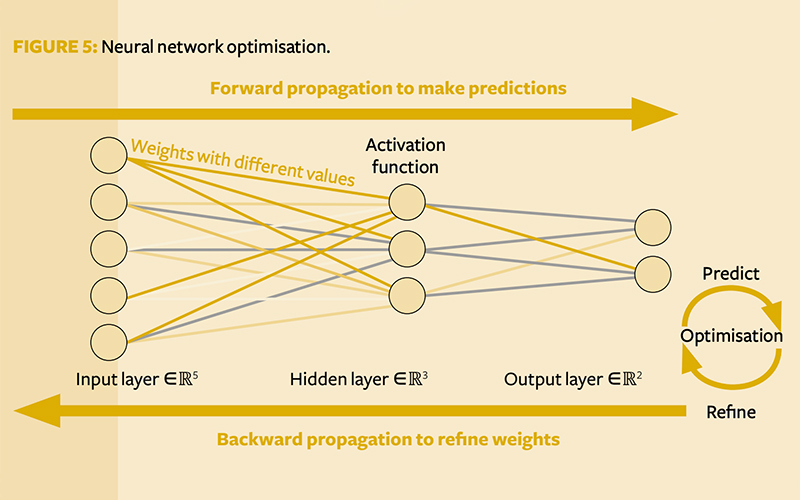
Neural networks are machine learning algorithms inspired by neuroplasticity models of the human brain. The structure of a feed-forward neural network resembles a layered cobweb with a series of input nodes on the left (input layer) that contain information from raw data. The output neuron nodes on the right (output layer) are the target we want to predict. A deep learning network would have one or more hidden layers of nodes in between to identify patterns and register interactions.

The hidden layers are the key component that allow neural networks to account for extremely complicated interactions. Each node in a hidden layer represents the aggregate information from raw data; the more nodes we have, the more relationships we are likely to capture.

Forward propagation happens when a neural network makes predictions from data, going from the left input layer to the right, and arrives at the output layer. But the algorithm does not end here, as accurate predictions do not come naturally just from the layered structure. To obtain good results, we need good weights linking the layers.

Apart from input nodes, neuron nodes in hidden and output layers are essentially the result of dot products from nodes in previous layers multiplying their corresponding weights, linking the next layer. Therefore, a proper set of weighting values is vital to improve prediction accuracy.

Backward propagation is used to optimise the weights for a given loss function. As the name suggests, it goes in the opposite direction to the forward propagation, starting from the prediction on the right and going all the way back to the input nodes on the left, calculating the gradients of the loss function based on error terms at each node. It then proposes an updated version of weights using gradient descent to minimise a given loss function. The algorithm then takes the updated weights and forward propagates again to achieve a new prediction, hopefully giving a smaller prediction error. Then the neural network backwards propagates to make yet another update for the weights. This iteration goes repeatedly over a complete set of data (‘epochs’) until the optimisation cannot be improved any further and the final prediction is achieved.

Off-the-shelf deep learning packages such as Keras are available in Python to execute the gradient descent method for us, so that we can build neural networks and get results quickly and easily. We set a simple neural network with two hidden layers that had 1,000 nodes in each. This produced a prediction with RMSE 0.2356 on the training set, 0.2380 on the testing set.

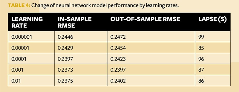
To optimise the model performance, we can experiment and search for the best learning rate, as can be seen in Table 4.

The learning rate represents the size of each update of weights. By comparison, the prediction performance keeps improving as the learning rate increases up to 0.001, then starts to drop a little when the learning rate grows beyond 0.01. This shows that the size of the update is too small to make a meaningful improvement when the learning rate is smaller than 0.001, but too large and leaps over the optimal point when it is larger than 0.001.

Many more experiments can be done to fine-tune neural networks, including but not limited to using different optimisers or hidden layers, differing the number of nodes, and changing associated activation functions. Neural networks are very flexible models, and it is important to be mindful about overfitting when adjusting them to suit customised purposes.

Naive bayes
Finally, a naive Bayes Bernoulli formula was used as a prediction of frequency. Naive Bayes has been shown to be a good estimator for imbalanced probabilistic problems.

The classifier is limited to binary outcomes, so prediction of more than one claim is lacking. The testing data RMSE turned out to be 0.2502, which is not ideal. We also tried to bucket all non-zero claim frequencies together to create a binary label, but the performance returned was worse, so it was dropped.

While naive Bayes has delivered many strongly performing models in use cases such as separating normal emails from spam and sentimental analysis applications, its claim frequency prediction accuracy falls short of expectations.

Thanks to the IFoA Data Science Research Section’s supervised learning workstream. Team members: Neptune Jin (lead), Usenthini Rajasekar, Jonathan Bowden, Tom Lambert, Hemant Rupani.

Results
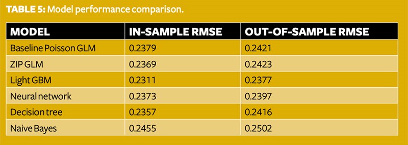
A table of comparison between the baseline model and the strongest candidate from each genre of supervised learning algorithms crowned GBM as the best model, followed by the neural network as the runner-up. Apart from naive Bayes models, all others outperformed the basic Poisson GLM in predicting the claim frequencies.

This study shows the possible applications of a large variety of supervised learning techniques in general insurance. While some experiments outperformed others, in this example there was by no means a one-size-fits-all recipe. Actuarial professionals are encouraged to expand their toolkits and be ready to pick up the best fitting algorithms.

Neptune Jin is a senior statistical analyst from BGL group