From raw to processed tweets

This is part of a series of posts that aim to explain in greater detail the NLP pipeline supporting the twitter sentiment analysis performed here.

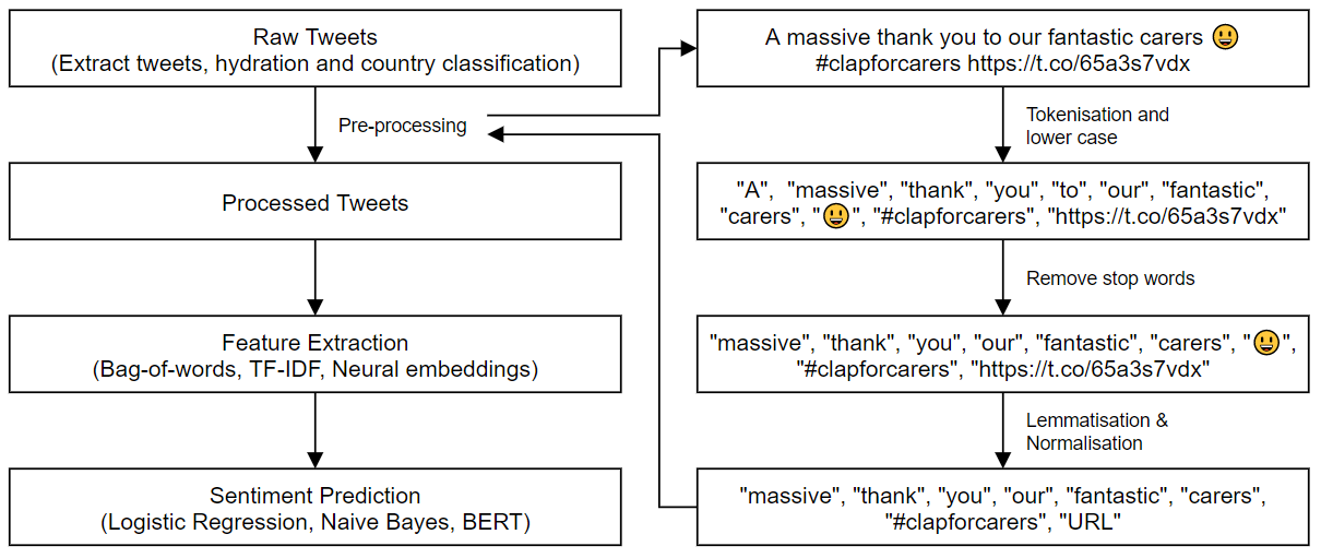
Step 1: Tweets pre-processing and reading in the data

Before the tweets can be used, we have to perform a few critical pre-processing steps:

1. Normalization, where we reduce randomness in the text by normalising irrelevant expressions, such as numbers, usernames and URL;
2. Removing stop words such as “to”, “the” and “my”; and
3. Lemmatization, where we reduce a word to its most meaningful base form.

These steps are summarised below in another python notebook.

stopwords = ['to', 'the', 'my', 'and', 'is', 'it', 'for', 'in', 'of', 'im', 'on', 'i',
            'me', 'so', 'that', 'just', 'with', 'be', 'at', 'a', 'i', 'its', 'this', 'was']

def normalize(text):
    """
    Normalize tweets to reduce randomness in text
    Arguments:
        text {str} -- Extracted "dirty" tweets
    Returns:
        text {str} -- Normalized tweets
    """
    text = re.sub(emoji.get_emoji_regexp(), r"", text)  # remove emojis
    text = re.sub(r'[0-9]+', 'NUMBER', text)  # remove numbers
    text = re.sub(r'@[A-Za-z0-9_]+', 'USER', text)  # remove @ username
    text = re.sub(r'https://[A-Za-z0-9./]+', 'URL', text)  # remove HTML
    text = re.sub(r'http://[A-Za-z0-9./]+', 'URL', text)  # remove HTML
    text = re.sub(r'\n', ' ', text)  # remove new line breaks
    text = re.sub(r'(.)\1+', r'\1\1', text)  # remove repeated characters beyond 2 letters

    text = "".join([char for char in text if char not in string.punctuation])  # remove punctuation

    text = text.strip()
    text = re.sub(' +', ' ', text)  # remove additional blank spaces

    return text

def clean(text):
    """
    Cleanse tweets by converting to lower case, remove stop words, lemmatize, normalise and remove
    empty items
    Arguments:
        text {str} -- Extracted "dirty" tweets
    Returns:
        text {str} -- Cleansed tweets
    """
    # lower case
    text = text.lower()
    text = re.sub(r'’', "'", text)  # clean apostrophes

    # tokenize
    text = tweet_tokenizer.tokenize(text)

    # Remove stop words
    text = [t for t in text if t not in stopwords]  # remove stopwords

    # Lemmatization
    text = [lemmatizer.lemmatize(x) for x in text]

    # Normalization
    text = [normalize(x) for x in text]

    # Remove empty items
    text = [x for x in text if x]

    # De-tokenize and convert back into string
    text = TreebankWordDetokenizer().detokenize(text)

    return text

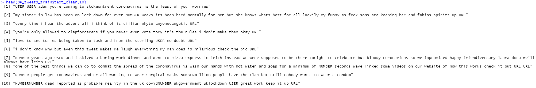
Finally, we can read in the raw tweets that has now been cleansed. Two minor additional processing steps are performed to substitute “’” and “-“ from the tweets.

A sample output from DF_tweets_train$text_clean is shown below.

DF_tweets_train <-  read_excel(paste0(path_dir, "\\tweets_train.xlsx"))
text_processed_train <- DF_tweets_train$text_clean

## Remove curly apostrophe (additional processing)
text_processed_train <- gsub("'", "", text_processed_train)
text_processed_train <- gsub("-", "", text_processed_train)

Step 2: Pruning the vocabulary

Prior to pruning the vocabulary, we need to prepare an iterator object which can be used as input into create_vocabulary(). Here, we also apply “tolower” to preprocessor, converting all letters to lowercase as well as tokenizing our tweets by word. This breaks up the tweets into individual words. Other possible alternatives include “space_tokenizer” or “stem_tokenizer”. More details can be found in the text2vec RDocumentation here.

it_train <- itoken(text_processed_train, 
                   preprocessor = tolower, 
                   tokenizer =  word_tokenizer,
                   n_chunks = 10,
                   progressbar = FALSE
)

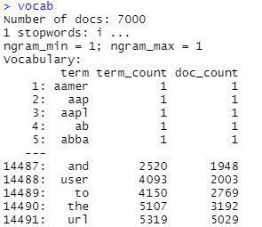
Once we have the iterator object, we can now count the appearance of each unique word using create_vocabulary(). We also filtered out stopwords in this step and selected 1-gram as an extraction criteria. This means that in the vocab dataframe, we will only see term_count and doc_count for single words.

term_count is defined as the number of times a particular word appears throughout all documents (or tweets), while doc_count is the number of documents (or tweets) in which that word appeared in. It comes as no surprise that the words “and”, “to” and “the” appeared the most often in tweets as shown below.

stop_words = c("i")
vocab <- create_vocabulary(it_train,
                           ngram = c(1,1),
                           stopwords = stop_words
) ## 14492

We then pruned the entire list of vocabulary using prune_vocabulary() which filters the input vocabulary and throws out very frequent and very infrequent terms. More details can be found in the text2vec RDocumentation here.

An important decision here was to select the parameters for which a word would be retained based on:

1. the minimum number of occurences over all documents (term_count_min)
2. the minimum number of documents containing this term (doc_count_min)
3. the maximum proportion of documents which should contain this term (doc_proportion_max)
4. the maximum number of terms in vocabulary (vocab_term_max). Note that this is to limit the absolute size of the vocabulary and does not have an effect here as it is set to the original number of rows.

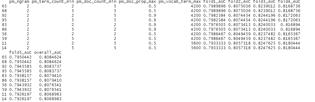
This decision was arrived at after performing a 5 fold cross validation over a total grid space of 108 cells, each representing a unique combination of each of the above parameters. The optimal combination was then selected based on AUC, as shown below. The cross validation steps are similar to what is presented in steps 1 to 3 here, except that these steps are applied to different folds of the data and based on unique combination of input parameters for prune_vocabulary(). The algorithm used in cross validation is glmnet.

# parameters derived from cross-validation above
pruned_vocab <- prune_vocabulary(vocab, 
                                 term_count_min = 2, 
                                 doc_count_min = 2,
                                 doc_proportion_max = 0.9,
                                 #doc_proportion_min = 0.0001, 
                                 vocab_term_max = nrow(vocab)
) ## 6144

Step 3: Creating a Document Term Matrix (DTM)

A DTM describes the frequency of terms that occur in a collection of documents (defined as individual tweets in our case). This is represented in a matrix form where

1. each row represetns one document (or tweet)
2. each column represents one term or word
3. the value in each matrix cell represents the number of times it appeared in that document (or tweet)

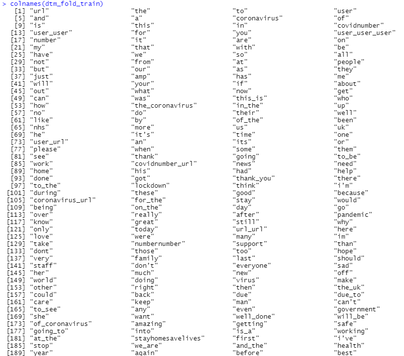
An example of a DTM is shown below, with the corresponding column names.

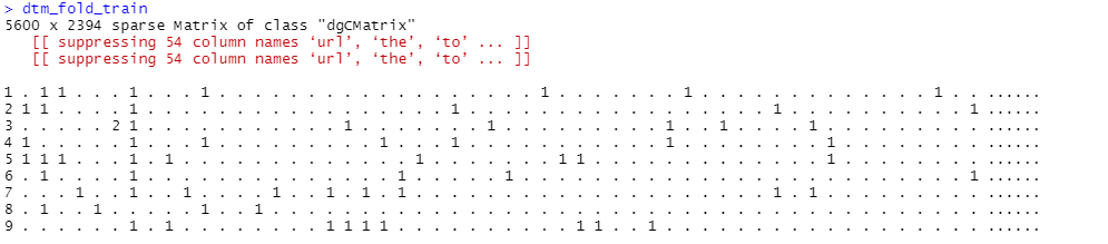
This is the base data structure which will be used as input in the modelling stage, after a transformation with TF-IDF in the next step. DTMs are often stored as a sparse matrix object, which is a matrix in which most of the elements are zero. This is a more efficient data structure compared to using standard dense-matrix structure, requiring less storage [1].

## Vectorisation - transform list of tokens into vector space
vectorizer <- vocab_vectorizer(pruned_vocab)

# create dtm_train with new pruned vocabulary vectorizer
dtm_train  <- create_dtm(it_train, vectorizer)
dim(dtm_train) ##7000x6141

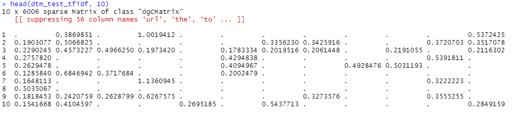
Step 4: Term Frequency Inverse Document Frequency (TF-IDF)

This final step is to compute TF-IDF from the DTM in step 3. TF-IDF consists of two metrics:

1. Term frequency of a word in a document (or tweet). For example, the word “and” appeared a cumulative 2520 times in our dataset.
2. Inverse document frequency of a word across all documents (or tweets). For example, the word “and” appeared in 1948 tweets our of 7000 tweets.

The higher the score, the more relevant that word would be in our dataset for that particular tweet.

At this point, we would have a matrix of TF-IDF scores (column) for each tweet (row) that we can then use as input when we train our model in the next step.

## fit the TF-IDF to the train data
tfidf <- TfIdf$new(smooth_idf = TRUE,
                   norm = "l2",
                   sublinear_tf = FALSE)
dtm_train_tfidf <- fit_transform(dtm_train, tfidf)

# apply pre-trained tf-idf transformation to test data
dtm_test_tfidf  <- create_dtm(it_test, vectorizer)
dtm_test_tfidf  <- transform(dtm_test_tfidf, tfidf)

For more information on the steps above, please refer to here.